Getting The Most Out of Excel - Our Top 10 Tips

Want to revolutionise the way you use Excel? Excel allows people to create, analyse and organise data using rows and columns in a rectangular grid. It provides the use of formulas, and automated calculations and enables data manipulation to assist in analysing the data created.

Here are our top 10 tips and tricks for 2024 to help you get the most out of Excel.

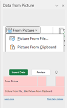
Add data from the internet (e.g. Table)

If you find data on the internet that you would like to transfer into a table in Excel, you can do so by following the below steps:

1. Right-click image, copy, and go to Excel.
2. Click on the Data Tab.
3. Select the From Picture dropdown box. 
4. Select Picture From Clipboard.
5. Excel will analyse the data, click on insert data once the analysis is complete and your data will appear in Excel. Note: You will be responsible for validating the accuracy of the data once copied and this may require additional formatting.  

Conditional Formatting

When looking at a large range of data it can be difficult to distinguish what you are looking for, i.e. highest to lowest numbers or percentages. Conditional formatting allows you to highlight these by colour-coding cells.  To do this, simply:

1. Select the cells you would like to format.

2. Click on the Home Tab and select Conditional Formatting.

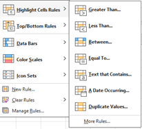
3. From the dropdown menu list, select the type of rule you want to apply. You can choose to highlight cells that contain a value Greater or Less than using the Highlight cells rule, select percentages using the Top/Bottom rules, add gradient fills using data bars and much more.

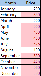
4. Here we have chosen to highlight data “Greater Than”. Simply click on the Greater than icon and the greater than dialogue box will appear. Type in the value you would-like to format by e.g. 330 as per the example below.

5. You can then choose to format this value by colour by selecting this in the With dropdown box as seen in the screenshot above.

6. Click OK to apply this rule and your data will appear colour-coded by the value greater than what you have selected.   

Autofill

If you are filling in multiple cells with a continuation of data e.g. Months of the year, you can use the Autofill button to drag down/across and autofill the remaining cells of an Excel spreadsheet, rather than manually typing this data in. To do so:

1. Type the data into the first cell you want to use as a basis for filling additional cells.
2. A small green box will appear in the bottom right of this cell when selected. Hover your mouse over this green box until a black cross appears (fill handle) and use your mouse to drag this arrow across the remaining cells you would like to automatically fill.

Autofill can be used for a range of values e.g. numerical dates/numbers etc.

Automatically Adjust a Column to Fit Your Data

No more double-clicking the top of each cell to manually adjust the width of your column to fit the data you have just typed in. You can set the column to automatically adjust as you type by selecting the below:

1. Right-click on Worksheet Tab

2. Select View Code

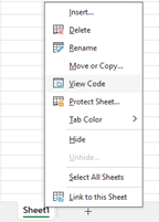
3. Select Worksheet from the drop-down box.

4. Type in the code Cells.Entirecolumn.AutoFit into the worksheet.

5. Close the window and go back to your worksheet and your columns will autofit your text automatically.

Selecting Data & Text in Cells

You can quickly and easily select a dataset using the below keyboard shortcut, rather than using your mouse and dragging the cursor, especially in a spreadsheet that contains 100’s of rows and columns.

1. Click in the first cell you want to select and hold down Ctrl + Shift then arrow up, down, left or right for the direction you want to select your text.
2. If you select Ctrl + Shift + End the cursor will jump to the lowest right-hand cell data, selecting everything in between.
3. Ctrl + Shift + * might be even faster, as it selects the whole contiguous data set of the worksheet, stopping at cells that are blank.

Split Text Function with Delimit

At times you may need to split data between multiple columns, which Excel allows you to do without manually typing this in. For example, you might need to split a client’s first and last name into 2 separate columns or separate a company name from the company email address.

1. Select the column you want to split.

2. Select the Text to Columns option from the Data

3. A dialogue box will appear with an option for “Delimited”.  

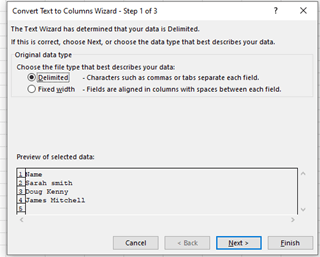
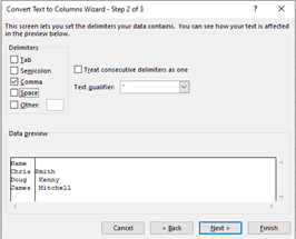
4. Delimit – lets you break up the column based on characters such as space, commas etc. You will need to select the character present in your data e.g. Chris, (Comma) Smith.

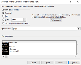
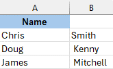
5. Once selected, click on next and enter the destination cell for the split data. In this instance, it will be Column 1 ($A$1) and click finish. The data will appear split as per the example below.

Recommended Pivot Tables

Pivot tables allow you to summarise, analyse, explore, and present data. They allow you to easily see comparisons, patterns and trends and are useful to help you make informed decisions about your compiled critical data.

1. Select the data range you want to insert a pivot table from.

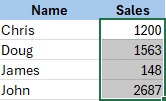
2. Select the Insert Tab and click on Recommended Pivot Tables.

3. Review the suggested options in the review pane.

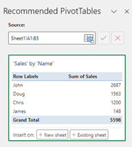
4. Select either +New or +Existing Sheet to insert the selected pivot table into your workbook.

Search the Menu’s Feature

With so many different commands available for use in Excel, it can be difficult remembering where to find these in Excel’s menu tabs. Excel has inserted a new feature called “Search the Menu’s” that will help you to locate the command you are looking for. Simply:

1. Highlight the data cells you want to manipulate.

2. Right-click and type in the command you would like to use in the Search the menus box e.g. Rotate.

3. Select the command and Excel will action this in your workbook.

Cleaning Data Sheets

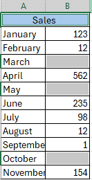
It is important to ensure all data in your worksheet is accurate and up to date. This can help you avoid errors and any inconsistencies that may lead to incorrect results and analysis. The 2 methods below will assist you in cleaning the data sheets within your workbook.

Remove Blanks

1. Select the workbook, press CTL + G & click on Special.

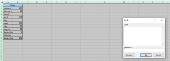
2. Select Blanks and OK. This will highlight any blanks found in your worksheet.

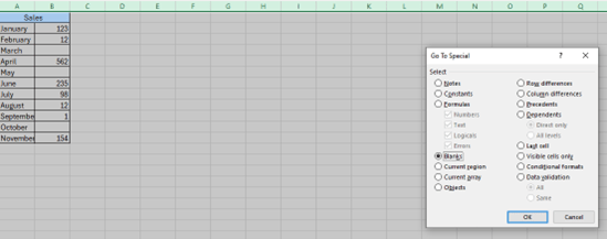
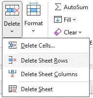
3. Go to the Home Tab, click on Delete and select rows to remove these.

Remove Duplicates

1. Go to the Data Tab.
2. Click on the Remove Duplicates icon.
3. You can select individual column categories and click ok to remove.

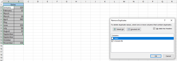
This will remove any duplicate cells.

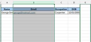
Move Columns within the Excel Worksheet

Did you know that you can move a column within your worksheet? This can help create a logical flow of information. To do so, simply:

1. Press the Shift key and click and hold the left mouse button.

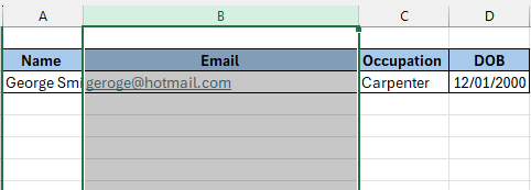
2. Select the left or right edge of the column you want to move and hover your mouse until an arrowed cross appears. Move your column to the desired new position.

By using the tips and tricks listed in this article, you will not only save time but learn new skills along the way.

If you & your team are interested in how to get the most out of Excel and Microsoft Office 365, get in touch, our team would love to help.